
Chapter 9 The Influence of Monetary and Fiscal Policy on Aggregate Demand
LEARNING OBJECTIVES学习目标:
understand the relation of fiscal policy and aggregate demand
explain the multiplier effect and crowding out effect
identify the difference between the multiplier effect and crowding out effect
FOCUS AND DIFFICULTIES知识重难点:
Focus: the concepts of multiplier effect and crowding out effect
Difficulty: distinguish between multiplier effect and crowding out effect
LECTURE VIDEO学习视频:
LEARNING OUTLINE学习大纲:
1. Fiscal Policy and Aggregate Demand
Definition of fiscal policy: the setting of the level of government spending and taxes by government policymakers.
When policymakers change the money supply or the level of taxes, they shift the AD curve indirectly by influencing the spending decisions of firms or households. While, when the government changes its own purchases of goods and services, it shifts the AD curve directly.
Expansionary fiscal policy including an increase in government spending or a decrease in taxes, shifts AD curve to the right.
Contractionary fiscal policy including a decrease in government spending or an increase in taxes, shifts AD curve to the left.
2. Changes in Government Purchases
Suppose that the U.S. Department of Defense places a $20 billion order for new fighter planes with Boeing.
It means an increase in government spending of $20 billion, thus increasing the aggregate demand. As a result, the AD curve shifts to the right.
A. The Multiplier Effect
(1)
When the government buys $20 billion of planes from Boeing, the immediate impact is to raise the revenue and employment at Boeing.
Then, as the Boeing's wokers see higher wages and owners see higher profits or dividends, they also as consumers, will likely increase their consumption spending.
As a result, this extra consumption causes further increases in aggregate demand.
So, we realize that the initial $20 billion increase in government spending can raise the AD by more than $20 billion because in addtion to increasing government spending, expansionary fiscal policy increases income and thereby increases consumer spending. This is known as multiplier effect.
(2)
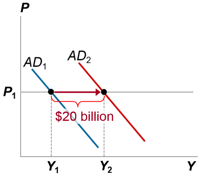
The increase in government spending of $20 billion initially shifts the AD curve to the right by exactly $20 billion. (AD1→AD2)
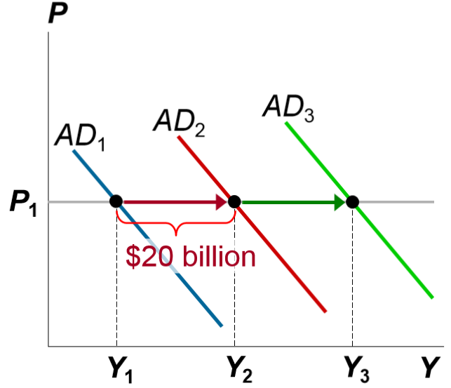
But when consumers respond by increasing their consumption spending, the AD curve shifts furtuer to the right. (AD2→ AD3)
So, the total spending rises by more than the initial increase in government purchases, because of the multiplier effect.
(3) Marginal Propensity to Consume
The size of multiplier effect depends on by how much consumers would increase their spending in response to increases in income.
Marginal propensity to consume (MPC): the fraction of extra income that households consume rather than save.
where C is the consumption spending and Y is the total income,
is the changes.
If MPC= 0.8 and income rises $100, consumption rises by $80 (=0.8*100).
Since: Y = C + I + G + NX
Y refers to both the total spending (namely AD) and total income, in terms of GDP.
I and NX are assumed to be unchanged.
ΔY = ΔC + ΔG ;
Because MPC=ΔC/ΔY , substituting the ΔC with MPCΔY.
So, ΔY = MPC ΔY + ΔG;
And, , where
refers to the multiplier.
Note that the size of the multiplier depends on the size of the marginal propensity to consume.
With a larger MPC, people consume more in response to a rise in income, which inturn cause a bigger rise in aggregate demand.
(4)
Because of multiplier effect, a dollar of government purchases can generate more than a dollar of AD.
The logic of the multiplier effect is not restricted to changes in government purchases. It applies to any event that changes the consumption, investment, government purchases, or net exports.
For instance, a economic boom overseas increases the nation's net exports. This increase on net exports increases national income, which in turn stimulates more consumption spending.
A stock market boom makes household wealthier and increases their consumption spending. This extra consumption spending increases national income, which in turn leads to more consumption spending.
So, the multiplier effect can amplify the impact of changes in any spending component of GDP.
A small initial change in consumption, investment, government purchases, or net exports can end up with a larger effect on AD and therefore, the economy's total output.
B. The Crowding-Out Effect
When an increase in government spending raises the AD for goods and services, it also causes the interest rate to rise, which reduces investment spending and reduces the initial increase in AD.
The reduction in AD that results when a fiscal expansion raises the interest rate and thereby reduces investment spending, is called the crowding out effect.
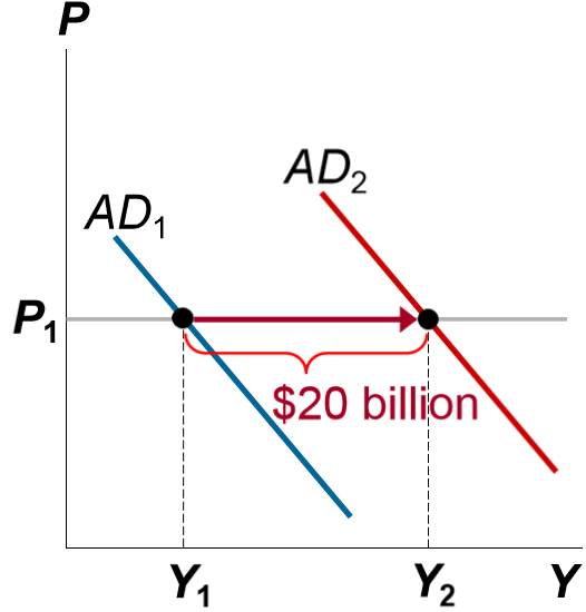
When the U.S. government buys $20 billion new planes from Boeing, the $20 billion increase in government spending initially shifts AD to the right by $20 billion. (AD1→AD2)
Note: This graph demonstrates the crowding-out effect in isolation, ignoring the multiplier effect.
As Boeing's workers see higher wages and owners see higher profits, they plan to buy more goods and services, as a result, need hold more of their wealth in terms of money. That is, the increase in income caused by the fiscal expansion raises the money demand. (MD1→MD2)
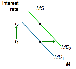
As shown in the money market, when the higher income shifts the MD curve to the right, the interest rate must rise and in turn reduces the investment spending. (AD2→AD3)
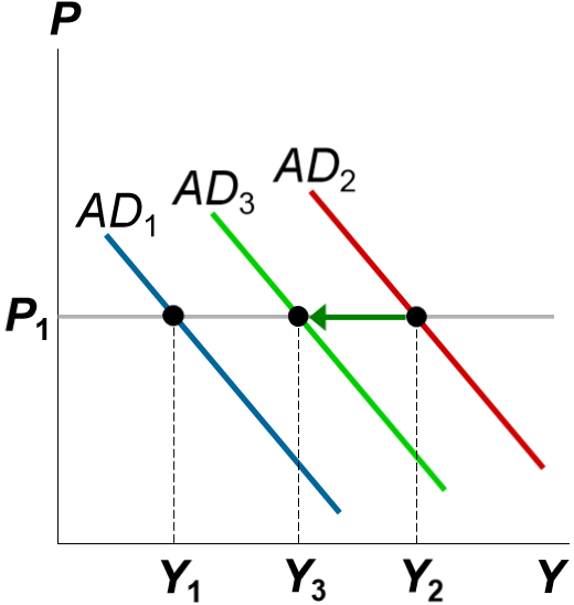
Thus, even though the increase in government purchases shifts the AD curve to the right initially, this fall in investment spending will then pull AD back toward the left.
Thus, aggregate demand ultimately increases by less than $20 billion---the initial increase in government spending.
Therefore, when the government increases its purchases by $X, the aggregate demand for goods and services could rise by more or less than $X, depending on whether the multiplier effect or the crowding-out effect is larger.
If the multiplier effect is greater than the crowding-out effect, aggregate demand will rise by more than $X.
If the multiplier effect is less than the crowding-out effect, aggregate demand will rise by less than $X.
3. Changes in Taxes
If the government reduces taxes, households will likely spend some of this extra income, shifting the aggregate-demand curve to the right.
If the government raises taxes, household spending will fall, shifting the aggregate-demand curve to the left.
The size of the shift in the aggregate-demand curve will also depend on the sizes of the multiplier and crowding-out effects.
Another important determinant of the size of the shift in aggregate demand due to a change in taxes is whether people believe that the tax change is permanent or temporary. A permanent tax change will have a larger effect on aggregate demand than a temporary one.

