Chapter 8 Aggregate Demand and Aggregate Supply

LECTURE VIDEO学习视频(6):

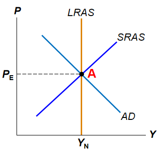
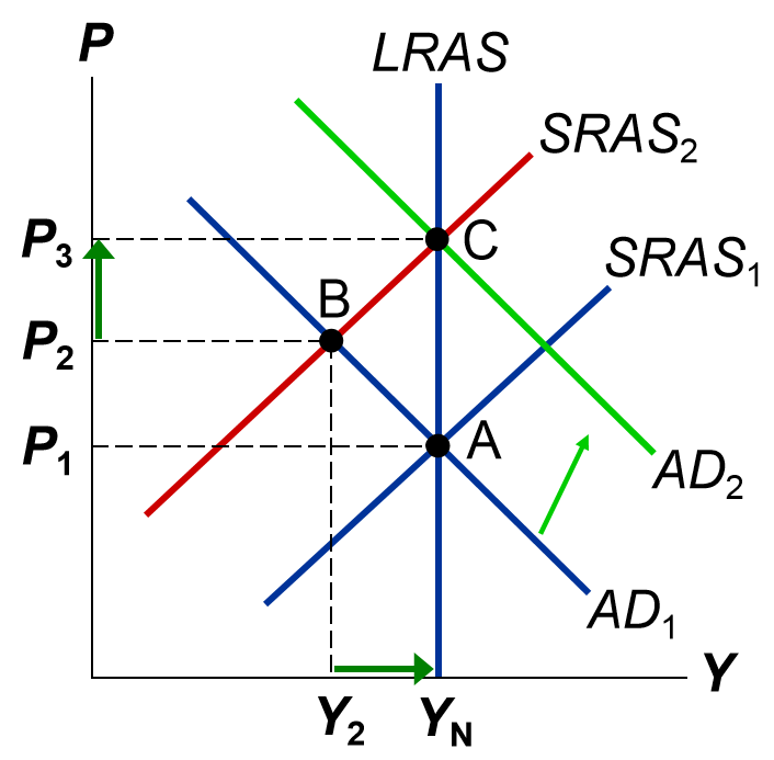
Long-Run Equilibrium

The long-run equilibrium of the economy is achieved where the AD curve crosses the LRAS curve, at point A, P=, Y=, and uneployment is at its natural rate.

When the economy reaches this long-run equilirium, the actual price level equals the expected price level. As a result, the SRAS curve crosses this point as well.

The Effects of a Shift in Aggregate Demand

Assume the economy begins in long-run equilibrium, represented by point A in the graph, where the expected price level equals the actual price level (=), the output equals the natural rate of output (Y=)

Example: a stock market carsh sharply, reducing consumers' wealth.

(1) This event depresses consumers' spending. So, the AD curve shifts to the left.  

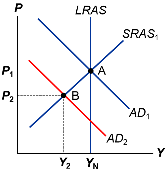
(2) The economy reaches a new short-run equilibrium at point B, where the new AD curve and the initial SRAS curve intersect. 

As the economy moves from point A to point B,  the price level falls and output falls, hence unemployment is higher. A declining output indicates that the economy is in recession. 

Thus, in short run, a stock market crash causes shifts in AD and leads to falling incomes and rising unemployment.

(3) Before the stock market crash, people expect the price level to be "" in the begining.

After the stock market crash, the actual price level immediately drops below the expected price level (<=).

People may not adjust their expectations of price level immediately, but over time, to catch up with the new reality, people adjust their expectations, lowering the expected price level.

When the expected price level declines, the SRAS curve shifts to the right until the economy reaching a new long-run equilibrium, point C, where the output is back to its natural rate and the price level drops further, but expectations catch up to reality P= once again.

Thus, in the long run, shifts in AD do not affect output but influence the price level.

Implications:

As we can see here, in the short run, expectations are fixed and the economy finds itself at the intersection of the AD curve and the SRAS curve. In the long run, if people observe that the price level is different from what they expected, their expectations adjust and the SRAS curve shifts. 

This shfts ensures that the economy eventually finds itself at the intersection of the AD curve and the LRAS curve. Thus, the influence of the expected price level on the position of the SRAS curve plays a key role in explaining how the economy makes the transition from the short run to the long run.

Moreover, we can notice that, in the absence of policy intervention, the economy “self-corrects.”  Of course, this process takes time, and policymakers may not want to wait.  At point B, policymakers could use expansionary fiscal or monetary policy to shift aggregate demand to the right and move the economy back to A.  

4. Case study: 

(1) Two Big Shifts in Aggregate Demand

(a) The Great Depression

In the early 1930s, U.S. experienced a large drop in its real GDP, called the Great Depression, it is by far the largest economic downturn in U.S. history.

From 1929 to 1933, GDP fell by 27%, the unemployment rate rose from 3% to 25%, and the price level fell by 22% over these four years.

Two possible causes of the Great Depression:  the fall in the money supply, and the stock market crash. 

From 1929 to 1933, U.S. money supply fell by 28% and stock pricees fell about 90% during this period, thereby depressing investment spending and consumer spending.

Either would shift the AD curve left, causing P and Y to fall and causing unemployment to rise. 

(b) World War II

The economic boom of the early 1940s was clearly caused by a sharp rise in U.S. govt spending during the World War II.

As the U.S. government devoted more resources to the military, government purchases of goods and services increased almost fivefold from 1939-1944.

Our model predicts an increase in G would shift AD to the right, increasing P and Y, and reducing unemployment. 

These predictions are consistent with the data: From 1939 to 1944, U.S. real GDP rose by 90%, the price level rose by 20%, and unemployment rate fell from 17% to 1%.

Thus, our model makes sense to explain some economic fluctuations.

(2) The Recession of 2008–2009

The United States experienced a financial crisis and severe economic downturn in 2008 and 2009.

The story of this downturn begins with a substantial boom in the housing market. 

After the recession in 2001 caused by the dot com bubble, the Fed lowered interest rates to historically low levels in order to help economy recover.

Low interest rates allow many low-income families to get a mortgage and buy a house, thus increasing the housing demand and also raising the housing prices.

From 1995 to 2006,  average housing prices in U.S. more than doubled.

However, from 2006 to 2009, housing prices fell about 30%. The price decline casued a sizable fall in aggregate demand.

Due to a sharp decline in housing prices, many homeowners stopped to paying their loans, so a large number of mortage defaults which make financial institutions that owned mortgage-backed securities suffered huge losses.

As a result of all these events, the U.S. experienced a large drop in aggregate demand causing real GDP to fall and unemployment to rise.

Real GDP fell sharply by 4% between the forth quarter of 2007 and the second quarter of 2009

Unemployment rate rose from 4.4% in May 2007 to 10.1% in October 2009

To return AD to its previous level, the U.S. government adopted three main policy actions.

First, the Fed lowered the target for the federal funds rate and conducted open market purchase to provide banks with addtional funds so that banks can recover its loan-making.

Second, the U.S. Treasury put $700 billion into banking system to increase the amount of bank capital and thus U.S. government – temporarily became a part owner of these banks.

Third, at that time the new U.S. president  Barack Obama signed a $787 billion stimulus bill, February 17, 2009, so as to increase the government spending.

5. The Effects of a Shift in Aggregate Supply

Assume the economy begins in long-run equilibrium

Example: Firms experience a sudden increase in their costs of production.

(1) Higher production costs make producing and selling goods and services less profitable, so firms supply a smaller quantity of output for any given price level.

Thus, the SRAS curve shifts to the left.  (Depending on the event, long-run aggregate supply may also shift. But, to keep things simple, we will assume that it does not.)

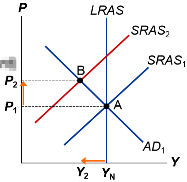
(2) In the short run, as the economy moves from point A to point B, output will fall and the price level will rise. The economy is experiencing stagflation.

Definition of stagflation: a period of falling output and rising prices.

(3) How stagflation affects nominal wages? Firms and workers at first respond to the rising price level by raising their expectations of the price level () and setting higher nominal wages. In this case, firms' labor costs will rise again, firms cut off more production and the SRAS curve would shift further to the left, making the staflation even worse. This phenomenon of higher prices leading to higher wages, inturn learding to higher prices, is called a wage-price spiral.

However, this process of rising wages and rising price level will slow down. Because, when firms reduce large production and fire more workers, the job hunters would be willing to accept a low level of wage because they have less bargining power when unemployment is high.

(4) So, eventually, nominal wages would fall, producing goods becomes profitable and the SRAS shifts to the right.

Until the SRAS curve back to the initial long run equilibrium, point A, the price level falls and the output is back to its natural rate.

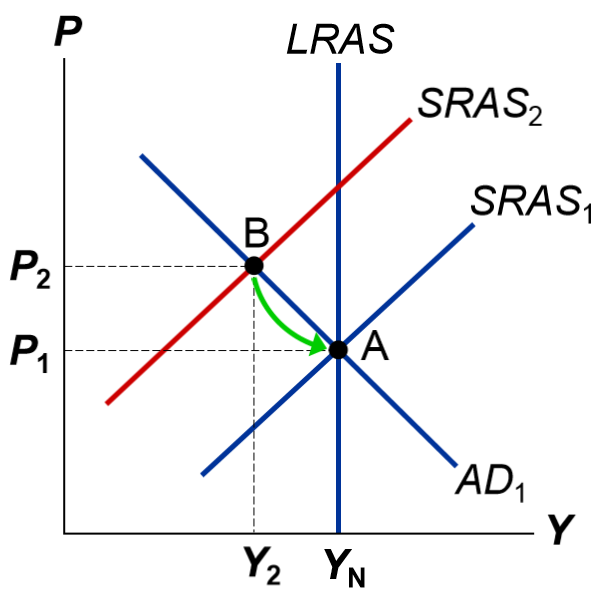
This transition back to the initial equilibrium assumes that AD is unchanged throughout the process.

Implication:

In the real world, if policymakers want to end the stagflation, they can use fiscal or monetary policy to increase AD and shift the aggregate-demand curve to the right, thus offsetting the effects of shifts in SRAS curve.

By doing this, the recession will end, the output returns to its natural rate, but the price level will be permanently higher.

6. Case study: Oil and the Economy

Crude oil is a key input in the production of many goods and services, and much of the world's oil comes from Saudi Arabia, Kuwait and other Middle Eastern countries.

When some event (often political) reduces the supply of crude oil and leads to a rise in the price of crude oil, firms must endure higher costs of production and the short-run aggregate-supply curve shifts to the left.

In the mid-1970s, OPEC lowered production of oil and the price of crude oil rose substantially. Oil-importing countries around the world experienced stagflation. The inflation rate in the United States was pushed to over 10%. Unemployment also grew from 4.9% in 1973 to 8.5% in 1975.

This occurred again in the late 1970s. Oil prices rose, output fell, and the rate of inflation increased.

Since OPEC is a cartel, which may fail to work when members cheat on aggreement.

In the late 1980s, OPEC began to lose control over the oil market as members began cheating on the agreement and supplying the crude oil. Oil prices fell, which led to a rightward shift of the short-run aggregate-supply curve. This caused both unemployment and inflation to decline.

However, in recent years, the world market for oil has not been as important a source of economic fluctuations. Part of the reason is that conservation efforts and changes in technology have reduced the economy's dependence on oil.