Chapter 8 Aggregate Demand and Aggregate Supply

LECTURE VIDEO学习视频(5):

5. Why the Aggregate-Supply Curve Slopes Upward in the Short Run

In the short run, the price level does affect the economy's output. Over the period of 1–2 years, an increase in P causes an increase in the quantity of g&s supplied.  As a result, the SRAS curve is upward sloping.

Theories – explain why the AS curve slopes upward in short-run:

(1) The Sticky-Wage Theory

Nominal wages are sticky in the short run and often slow to adjust to changing economic conditions due to long-term contracts between workers and firms along with social norms and notions of fairness that influence wage setting and are slow to change over time.

And, firms and workers usually fix the nominal wage in advance based on the expected future price level. Such a nominal wage might persist for three more years.

Example: 

Suppose a firm has agreed in advance to pay workers an hourly wage of $20 based on the expectation that the price level will be 100.

If the actual price level is 105, higher than the expected level.

It means each unit of product is sold at 105, 5% higher than firms had expected. Hence, firms get 5% more unit revenue for its output than expected.

While, labor costs are fixed at $20 per hour, resulting in a higher profit than expected. Thereby production is now more profitable, so firms increase its quantity of output supplied and hire more workers.

Conversely, if the actual price level is 95, lower than the expected level. 

It means each unit of product is sold at 95, 5% lower than firms had expected. Hence, firms receive 5% less unit revenue for its output than expected.

While, labor costs are fixed at $20 per hour, resulting in a lower profit than expected. Thereby production is now less profitable, so firms hires fewer workers and reduces the quantity of output supplied.

The sticky wage gives firms incentive to produce more when the actual price level turns out higher than expected (P>) and to produce less when the actual price level turns out lower than expected (P<).

Therefore, the SRAS curve slopes upward.

(2) The Sticky-Price Theory

Many prices of g&s are also sometimes adjusting slowly in response to changing economic conditions. this slow adjustment is part due to menu costs, the costs of adjusting prices.

Menu costs include the cost of printing and distributing new menues and the time required to change price tags.

As a result, prices as well as wages may be sticky in the short run and firms usually announce prices for products being sold in advance based on the expected future price level.

Example:

Suppose that after firms have annuouced their prices, the Fed increases the money supply unexpectedly which will increase the price level in the long run(ch30).

Based on such a belief, some firms without menu costs can respond by raising their prices immediately.

But, some firms with menu costs may not want to incur additional menu costs and so they lag behind in raising their prices.

Therefore, in the short run, these lagging firms are operated with relatively lower prices which attract more buyers and leads to a higher sales and thereby they hire more worker and increases production.

Conclusion:

Because not all prices adjust instantly to changing conditions. When the price level turns out to be higher than expected(P>), some firms may respond by increasing their prices immediately while some firms may lag behind, keeping their prices at lower-than-desired levels in the short run, which promote sales and cause firms to increase the quantity of goods and services supplied.

Conversely, when the price level turns out to be lower than expected(P<), some firms may respond by decreasing their prices immediately while some firms may lag behind, keeping their prices at higher-than-desired levels in the short run, which depress sales and cause firms to lower the quantity of goods and services supplied.

Hence, the SRAS curve slopes upward.

(3) The Misperceptions Theory

Changes in the overall price level can temporarily mislead suppliers about what is happening in the markets in which they sell their output. Firms may confuse changes in P with changes in the relative price of the products they sell.

Example:

Suppose the overall price level rises above the expected level.

An apple grower may notice a rise in its apple price before notice a rise in prices of many other products (like rice, noodles) the grower buy as consumers.

Thus, the grower mistakenly believe that as the price of apple rises while other product prices are unchanged, it is an increase in the relative price of apple to other products. Thus, the grower may then believe that the reward to apple production now has increased, and thus the grower increase the quantity of output supplied. 

Conclusion:

When P>, firms mistakenly believe that the relative prices of their products are rising, thus increasing output

When P<, firms mistakenly believe that the relative prices of their products are decreasing, thus decreasing output

So, the SRAS curve is upward-sloping.

(4) Summing Up

Economists debate which of these theories is correct and it is possible that each contains an element of truth.

For our purposes here, the similarities between these theories are more important than their differences:  all three imply that output in the short run deviates from its long-run level (the “natural rate of output”,) when the price level (P) deviates from the expected price level ().  

We introduce an equation of aggregate supply that shows how output deviates from natural rate of output when the actual price level is different than expected.  Y  =    +  a (P  –  ) 

When  P =,  Y = 

When  P < ,  Y < 

When  P > ,  Y > 

Notice that when the price level equals the expected price level, output is equal to its long-run value, the natural rate of output.  

In the short run, people may be fooled about the price level, or they may be locked into wages or prices that were set before they knew what the price level would actually be.  Hence, in the short run, P may differ from .  

But in the long run,  nominal wages will become unstuck, prices will become unstuck, and misperceptions about relative prices will be corrected. thus, in the long run, expectations catch up to reality, P = , and therefore  Y = , as in the Classical model. 

6. Why the Short-Run Aggregate-Supply Curve Might Shift

LRAS curve and SRAS curve are intersected at a point where the price level equals the expected price level, and the output equals the long-run level of output.

(1) Events that shift the LRAS curve will shift the SRAS curve as well.

Changes in labor, capital, natural resources, or technological knowledge

An increase in the economy's capital stock increases productivity, so both the long-run and short-run aggregate supply curves shift to the right.

A higher natural rate of unemployment decreases a economy's output in both the long-run and short-run, so both the long-run and short-run aggregate supply curves shift to the left.

(2) The expected price level will affect the position of the short-run aggregate-supply curve even though it has no effect on the long-run aggregate-supply curve.

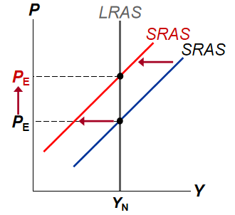
a) A higher expected price level decreases the quantity of goods and services supplied and shifts the short-run aggregate-supply curve to the left. 

For example, according to sticky wage theory, when wokers and firms raise their expectation of the price level, they are more likely to reach a labor contract with a higher level of nominal wages.

High wages increase firms' labor costs, thus reducing the profitability of firms' output. Therefore, firms decide to reduce the quantity of goods and services supplied at any given current price level.

So when the expected price level rises, wages are getting higher, costs increase, and firms produce less, causing the SRAS curve shift to the left.

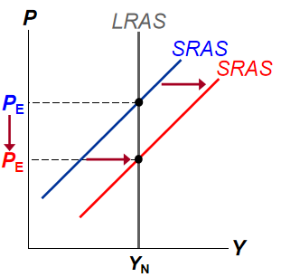
b) A lower expected price level increases the quantity of goods and services supplied and shifts the short-run aggregate-supply curve to the right.

When wokers and firms lower their expectation of the price level, they are more likely to agree with a lower level of nominal wages.

Lower wages decrease firms' labor costs, thus improving the profitability of firms' output. Therefore, firms will increase the quantity of goods and services supplied at any given current price level.

So when the expected price level decreases, wages are lower, costs decrease, and firms produce more, causing the SRAS curve shift to the right.