任务1.1:使用sklearn中的SVM实现手写数字识别。
| # 导入必备的包
import numpyas np
import struct
import os
# 定义加载所有训练数据集的函数
def load_mnist_train():
labels_path = 'mnist/train-labels.idx1-ubyte'
images_path = 'mnist/train-images.idx3-ubyte'
with open(labels_path, 'rb') as lbpath:
magic, n = struct.unpack('>II',lbpath.read(8))
labels = np.fromfile(lbpath,dtype=np.uint8)
with open(images_path, 'rb') as imgpath:
magic, num, rows, cols = struct.unpack('>IIII',imgpath.read(16))
images = np.fromfile(imgpath,dtype=np.uint8).reshape(len(labels), 784)
return images, labels
# 定义加载所有测试集数据集的函数
def load_mnist_test():
labels_path = 'mnist/t10k-labels.idx1-ubyte'
images_path = 'mnist/t10k-images.idx3-ubyte'
with open(labels_path, 'rb') as lbpath:
magic, n = struct.unpack('>II',lbpath.read(8))
labels = np.fromfile(lbpath,dtype=np.uint8)
with open(images_path, 'rb') as imgpath:
magic, num, rows, cols = struct.unpack('>IIII',imgpath.read(16))
images = np.fromfile(imgpath,dtype=np.uint8).reshape(len(labels), 784)
return images, labels
# 加载数据集
train_images, train_labels = load_mnist_train()
test_images, test_labels = load_mnist_test() |
| from sklearnimport preprocessing
# 60000个训练数据集
x = preprocessing.StandardScaler().fit_transform(train_images)
x_train = x[0:60000]
y_train = train_labels[0:60000]
# 10000个测试数据集
x = preprocessing.StandardScaler().fit_transform(test_images)
x_test = x[0:10000]
y_test = test_labels[0:10000] |
| # 加载svm机器方法
from sklearnimport svm
import time
print('开始训练....')
print(time.strftime('%Y-%m-%d %H:%M:%S'))
model_svc = svm.LinearSVC()
model_svc.fit(x_train,y_train)
print('结束训练....')
print(time.strftime('%Y-%m-%d %H:%M:%S')) |
| print('预测开始....')
y_pred = model_svc.predict(x_test)
print('10000个测试数据的测试准确率:')
print(model_svc.score(x_test,y_test)) |
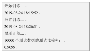
上述输出结果如图所示,准确率约为91%左右。训练线性SVM模型大约用时10分30秒。
也可以调用模型评估报告来查看,参考代码如下:
| from sklearn.metrics import classification_report
print(classification_report(y_pred, y_test)) |
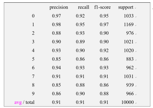
出具的更详细的模型评估结果如图9.6所示。其中,“0,4,6”的预测精确度相对较高。
任务1.2:可视化。
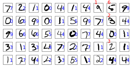
为更好地找到出错的图像用于分析,我们用不同颜色或位置来显示错误的预测结果。可视化显示预测结果与图片的对应关系,参考代码如下:
| import matplotlib.pyplotas plt
print('前100张测试图像的预测结果')
# 显示前100个样本的真实标签和预测值,用图显示
fig1=plt.figure(figsize=(8,8))
fig1.subplots_adjust(left=0,right=1,bottom=0,top=1,hspace=0.05,wspace=0.05)
for i in range(100):
# 用子图显示第i张图
ax=fig1.add_subplot(10,10,i+1,xticks=[],yticks=[])
ax.imshow(np.reshape(test_images[i], [28,28]),cmap=pltNaN.binary,interpolation='nearest')
# 在图上方显示预测结果值
ax.text(20, 20, str(y_pred[i]), color='blue',size = 20)
plt.show() |
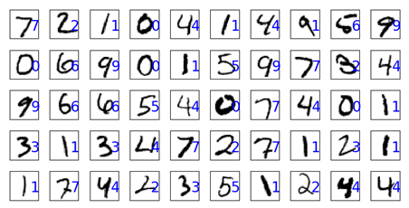
下图显示了前50张图片的具体预测结果。
任务1.3:为更好地找到出错的图像用于分析,我们用不同颜色或位置来显示错误的预测结果。
要求结果如图所示。
模型训练好后,我们就可以用它来做手写数字识别。当有新的手写体过来时,可以调用该训练好模型进行判别。
在机器学习模型中,需要人工选择的参数称为超参数。比如随机森林中决策树的个数,人工神经网络模型中的隐藏层层数和每层的节点个数,正则项中常数大小等等,它们都需要事先指定。超参数选择不恰当,就会出现欠拟合或者过拟合的问题。
我们在选择超参数有两个途径:一是凭经验;二是选择不同大小的参数代入到模型中,挑选表现最好的参数。通过途径二选择超参数时,人力手动调节注意力成本太高,非常不值得。For循环或类似于for循环的方法受限于太过分明的层次,不够简洁与灵活,注意力成本高,易出错。
GridSearchCV称为网格搜索交叉验证调参,它通过遍历传入的参数的所有排列组合,通过交叉验证的方式,返回所有参数组合下的评价指标得分。GridSearchCV实质是暴力搜索。该方法在小数据集上很有用,数据集大了就不太适用了。数据量比较大的时候可以使用一个快速调优的方法——坐标下降。它其实是一种贪心算法:当前对模型影响最大的参数调优,直到最优化;再拿下一个影响最大的参数调优,如此下去,直到所有的参数调整完毕。这个方法的缺点就是可能会调到局部最优而不是全局最优,但是省时间省力。
任务1.4:使用GridSearchCV为SVM寻找参数识别手写字体。
使用GridSearchCV调参考方法,训练SVM模型的参考代码如下:
| from sklearn.model_selection import GridSearchCV
# 调用GridSearchCV,为SVC()寻找最优参数
clf = GridSearchCV(SVC(class_weight='balanced'), param_grid={"C":[0.1, 1, 20, 10], "gamma":[0.01,5,0.1]}, cv=4)
# 用训练集训练SVC
clf.fit(x_train, y_train) |
同样,对于训练好的模型,可以对比一下,是否有更高的识别准确率。但是,在寻找最优参数过程相对耗时。