9.11 The Exponential Distribution

Another very common continuous distribution is called the exponential distribution. We can sample from the exponential distribution using the rexp() function. It takes two arguments:

• n: how many data points we want to sample

• rate: the rate that “successes” occur

rexp(n = 5, rate = 0.2)

## [1]  2.060884  7.210729  4.326803 31.713820  2.143409

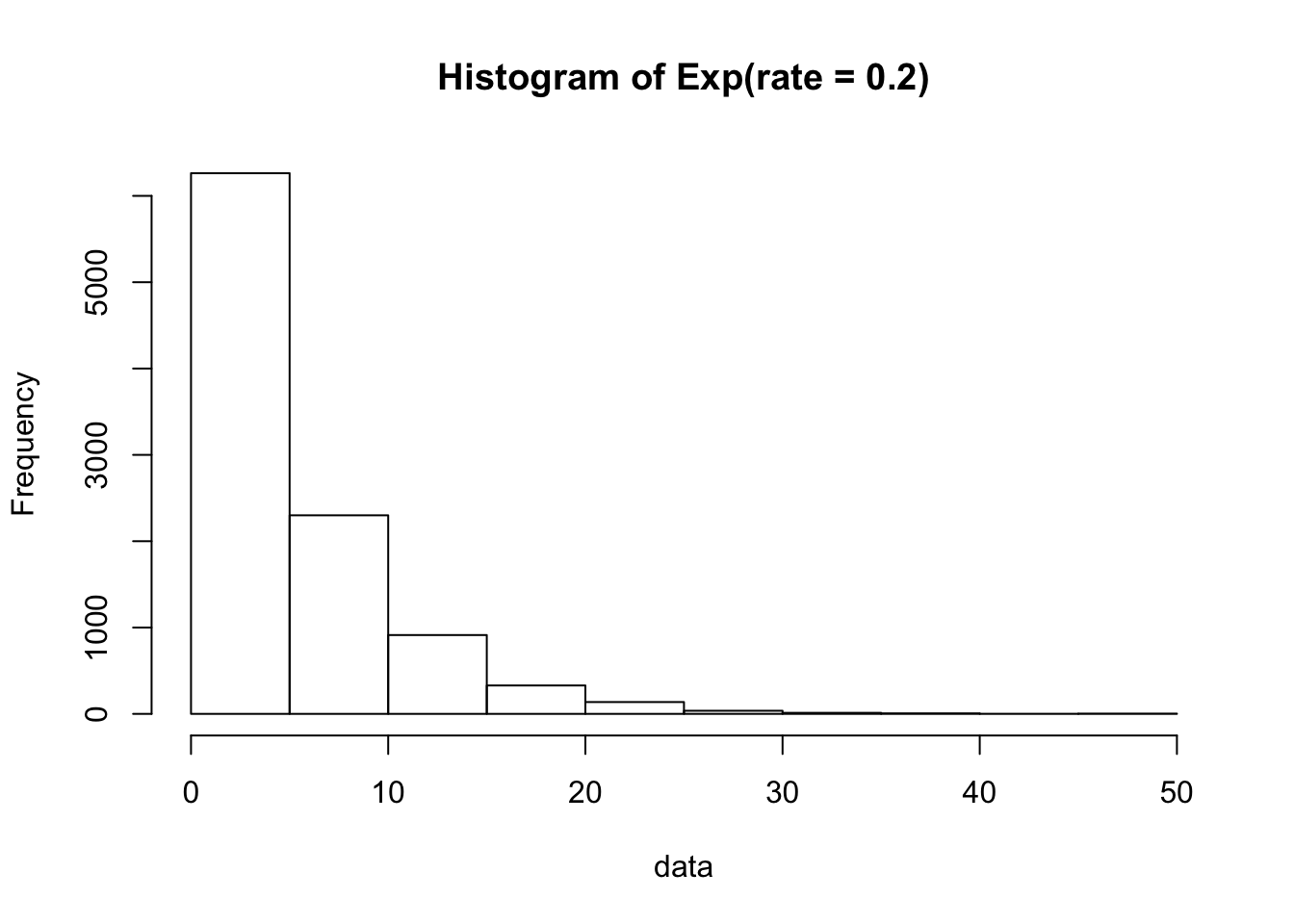
Since the exponential distribution is continuous, we use a histogram to plot the data. We sample 10,000 data points from this rate = 0.2 exponential distribution:

data = rexp(n = 10000, rate = 0.2)
hist(data, main = "Histogram of Exp(rate = 0.2)")

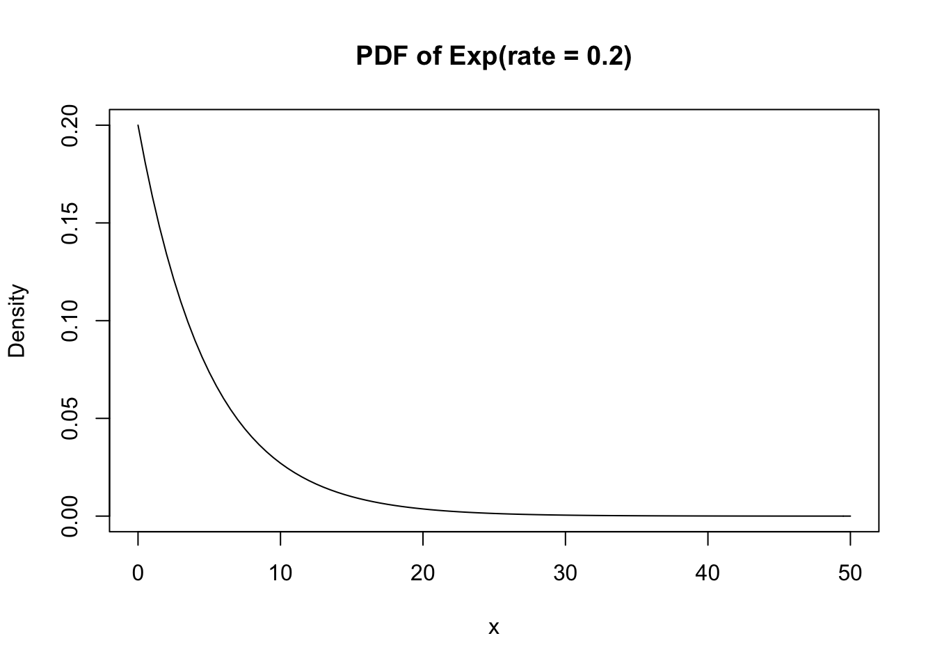
The exponential PDF can be plotted with:

curve(dexp(x, rate = 0.2), 
      xlim = c(0, 50),
      main = "PDF of Exp(rate = 0.2)", ylab = "Density")

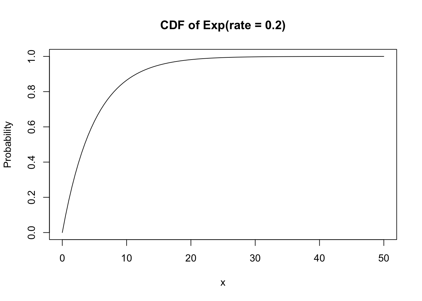
And the exponential CDF with:

curve(pexp(x, rate = 0.2), 
      xlim = c(0, 50),
      main = "CDF of Exp(rate = 0.2)", ylab = "Probability")