9.9 The Poisson Distribution

The Poisson distribution is a discrete distribution which was designed to count the number of events that occur in a particular time interval. A common (approximate) example is counting the number of customers who enter a bank in a particular hour. We traditionally call the expected number of occurrences $\lambda$ or lambda.

---

Poisson vs. binomial: The key difference between the Poisson and the binomial is that for the binomial, the total number of trials in the sample is fixed, while for the Poisson, the total number of events in the interval is not fixed. That said, the binomial distribution begins to look a lot like the Poisson distribution when the number of trials grows large, and the probability of success is small.

---

Random Samples: rpois

As with the binomial, we can easily sample from the Poisson using the rpois() function, which now take takes two arguments:

• n: how many outcomes we want to sample

• lambda: the expected number of events per interval

rpois(n = 10, lambda = 14)

##  [1] 12 14 18 13  9 13 10 17 20  8

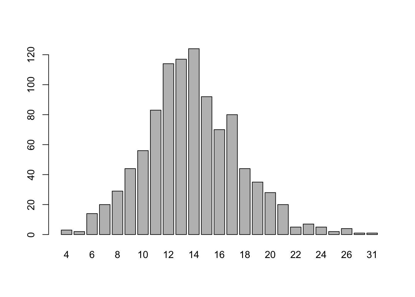
We can also plot a much larger sample of outcomes from this lambda = 14 Poisson distribution,

data = rpois(n = 1000, lambda = 14)
barplot(table(data))

Density Functions: dpois

The probability density function (PDF) of the Poisson distribution is given by:$$f\left(x|\lambda \right)=Pr(X=x)=\frac{{\lambda }^x{e}^{-x}}{x!}$$where $e$ is equal to 2.7182818 and $!$ is the factorial operator.

The function that computes this automatically is dpois(). The d stands for “density” and the pois stands for “Poisson”. Suppose we want to know the probability of getting 12 occurrences, we can get this easily with,

dpois(x = 12, lambda = 14)

## [1] 0.09841849

As before, we can easily obtain and graph the main part of the distribution,

barplot(height = dpois(0:30, lambda = 14), 
        names.arg = 0:30,
        main = "Poisson PDF", xlab = 'X', ylab = 'Probability')

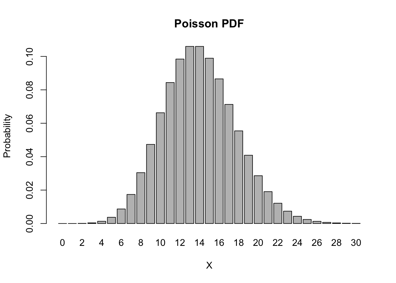
Note that this looks very much like the shape of the binomial distribution from the previous example. This is no coincidence, since the binomial(20, 0.7) and the Poisson(14) distributions are closely related (note that $20\cdot 0.7=14$).

Cumulative Distribution Functions: ppois

The cumulative distribution function (CDF) of the Poisson distribution is given by:$$F\left(q|\lambda \right)=Pr(X\le q)=\sum _{k=0}^{q}f\left(k|\lambda \right)$$

Suppose we want to know the probability of getting at most 12 occurrences, we can get this easily with,

ppois(q = 12, lambda = 14)

## [1] 0.3584584

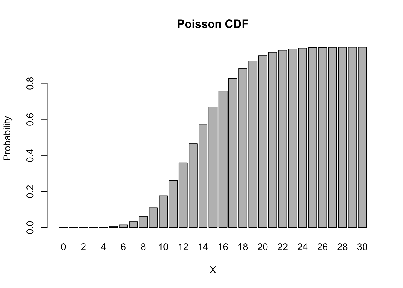
As before, we can easily obtain and graph the main part of the CDF,

barplot(height = ppois(0:30, lambda = 14), 
        names.arg = 0:30,
        main = "Poisson CDF", xlab = 'X', ylab = 'Probability')