9.8 The Binomial Distribution 二项分布

The binomial random variable is defined as the sum of repeated Bernoulli trials, so it represents the count of the number of successes (outcome=1) in a sample of these trials. The argument size in the binom functions tells R the number of Bernoulli trials we want in the sample.

Random Samples: rbinom

Notice we used the binom functions with size = 1 to explore the Bernoulli distribution above, so we just need to change this argument to sample from a binomial distribution:

rbinom(n = 15, size = 20, p = 0.7)

##  [1] 14 13 17 12 16 14 18 11 11 14 13 14 17 14 15

This represents the process of taking 15 samples, each with 20 trials, where the probability of success in each trial is 0.7, and the outcomes are the number of successes in each sample.

---

Note: In the traditional notation for the binomial PDF B(n,p), we write:$$P(X=k;n,p)=(\frac{n}{k})\left(p{)}^x\right(1-p{)}^{n-k}$$In this context $n$ refers to the number of (bernoulli) trials in the sample.
But in R, size is used to refer to the number of trials in the sample, and n is is instead used to refer to the number of outcomes you want to randomly draw from the binomial distribution.

---

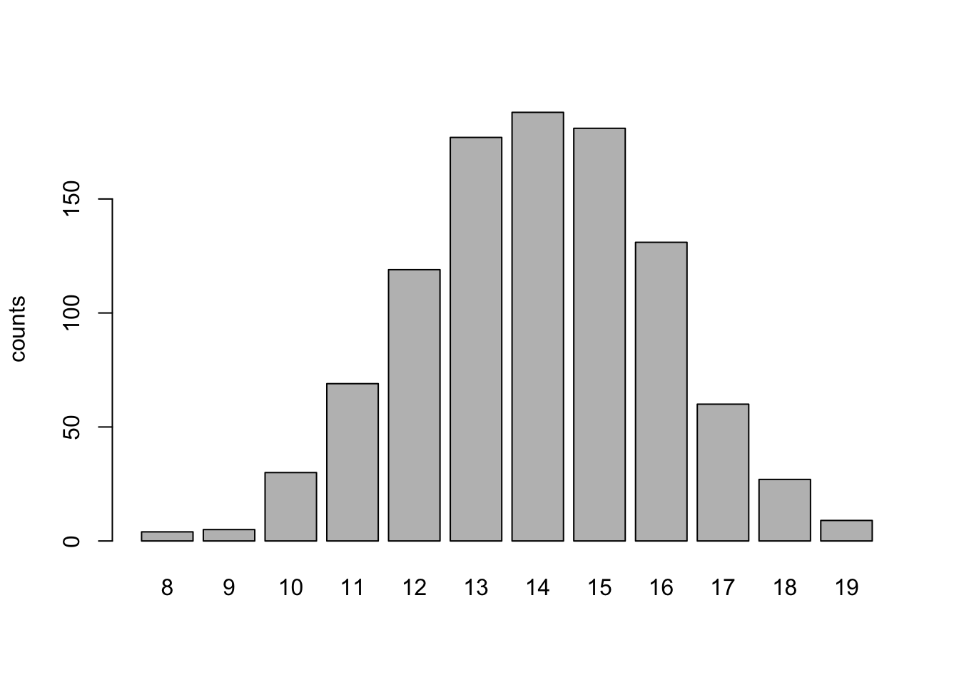
We can plot these outcomes if we simulate too many to examine directly,

dat <- rbinom(n = 1000, size = 20, p = 0.7)
barplot(table(dat), ylab = "counts")

Density Functions: dbinom

The probability density function (PDF) of the binomial distribution is given by:$$f(x|n,p)=Pr(X=x)=(\frac{n}{x})p^x(1-p{)}^{n-x}$$

The function that computes this automatically is dbinom(). The d stands for “density” and the binom stands for “binomial”. Suppose we want to know the probability of getting 12 successes in 20 trials, we can calculate this easily with,

dbinom(x = 12, size = 20, p = 0.7)

## [1] 0.1143967

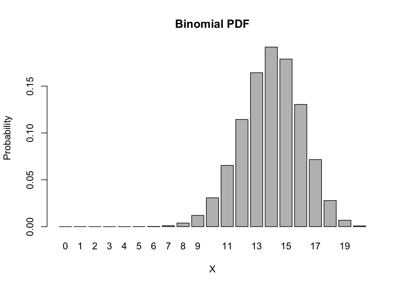
In fact, we can easily obtain and graph the probability of every possible outcome in this binomial distribution,

barplot(height = dbinom(0:20, size = 20, p = 0.7), 
        names.arg = 0:20,
        main = "Binomial PDF", xlab = 'X', ylab = 'Probability')

Cumulative Distribution Functions: pbinom

The cumulative distribution function (CDF) of the binomial distribution is given by:$$F(q|n,p)=Pr(X\le q)=\sum _{k=0}^{q}f(k|n,p)$$

Suppose we want to know the probability of getting at most 12 successes in 20 trials, we can obtain this easily with,

pbinom(q = 12, size = 20, p = 0.7)

## [1] 0.2277282

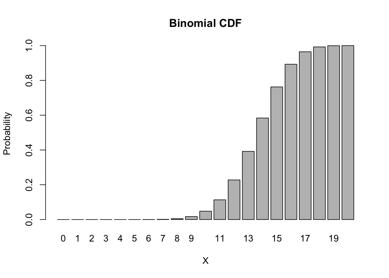
In fact, we can easily obtain and graph the entire CDF,

barplot(height = pbinom(0:20, size = 20, p = 0.7), 
        names.arg = 0:20,
        main = "Binomial CDF", xlab = 'X', ylab = 'Probability')

We can illustrate the relationship between the PDF and the CDF in the following plot,

par(mfrow = c(1,2))
barplot(height = dbinom(0:20, size = 20, p = 0.7), 
        names.arg = 0:20, 
        ylim = c(0,1),
        main = "Binomial PDF", xlab = 'X', ylab = 'Probability',
        col = c(rep("blue", 15), rep("gray", 8)))
barplot(height = pbinom(0:20, size = 20, p = 0.7), 
        names.arg = 0:20, 
        ylim = c(0,1),
        main = "Binomial CDF", xlab = 'X', ylab = 'Probability',
        col = c(rep("gray", 14), "blue", rep("gray", 6)))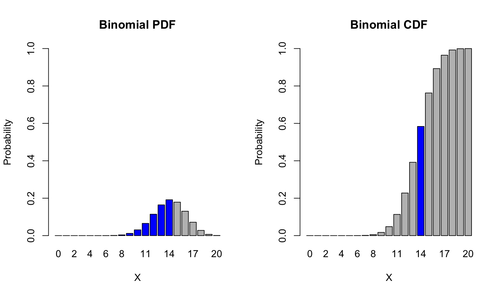

 Notice that the value of the CDF at $X=14$ corresponds to the sum of the PDF from $X=0$ to $X=14$.

Properties of Distributions

Note that the sum of the densities is,

sum(dbinom(0:20, size = 20, p = 0.7))

## [1] 1

And we can obtain the expectation of this binomial distribution, using the general definition: $\text{E}\left(X\right)=\sum x_i\cdot P(X=x_i)$

sum(0:20 * dbinom(0:20, size = 20, p = 0.7))

## [1] 14

Note that this is also what we get using the specific formula for the expectation of a binomial: $\text{E}\left(X\right)=np=20\cdot 0.7$.

The variance can be calculated using the general form: $\text{Var}\left(X\right)=\sum (x_i-\text{E}(X){)}^2\cdot P(X=x_i)$

sum((0:20 - 20 * 0.7)^2 * dbinom(0:20, size = 20, p = 0.7))

## [1] 4.2

Which is equal to specific formula for the variance of a binomial: $\text{Var}\left(X\right)=np(1-p)=20\times 0.7\times 0.3$.