There is a whole world of R functions we can use to sample random values from probability distributions or obtain probabilities from them. Generally, each of these functions is referenced with an abbreviation (pois for Poisson, geom for Geometric, binom for the Binomial, etc.) preceded by the type of function we want, referenced by a letter:

• r… for simulating from a distribution of interest

• d… for obtaining the probability mass function $P[X=x]$ (or probability density function for continuous random variables)

• p… for obtaining the cumulative distribution function, which is just a fancy way of saying $P[X\le q]$ for any value of $q$.

• q… for the quantile function of a distribution of interest

9.7.1 The Bernoulli Distribution 二项分布

A Bernoulli random variable ($X\sim \text{Bernoulli}\left(p\right)$) is equivalent to a (not necessarily fair) coin flip, but the outcome sample space is $\{0,1\}$ instead of heads and tails. The parameter $p$, by convention, signifies the probability of getting a 1, and a single draw of a Bernoulli random variable is called a “trial.”

Random Samples: rbinom

The best way to simulate a Bernoulli random variable in R is to use the binomial functions (more on the binomial below), because the Bernoulli is a special case of the binomial: when the sample size (number of trials) is equal to one (size = 1).

The rbinom function takes three arguments:

• n: how many observations we want to draw

• size: the number of trials in the sample for each observation (here =1)

• p: the probability of success on each trial

rbinom(n = 1, size = 1, p = 0.7)

## [1] 1

We can also randomly draw a whole bunch of Bernoulli (single) trials:

rbinom(n = 20, size = 1, p = 0.7)

##  [1] 0 1 1 1 0 0 1 1 0 1 0 1 1 1 1 1 0 0 1 1

Check out the help function for rbinom to see the arguments you can use with this function, and their meaning.

Density Functions: dbinom

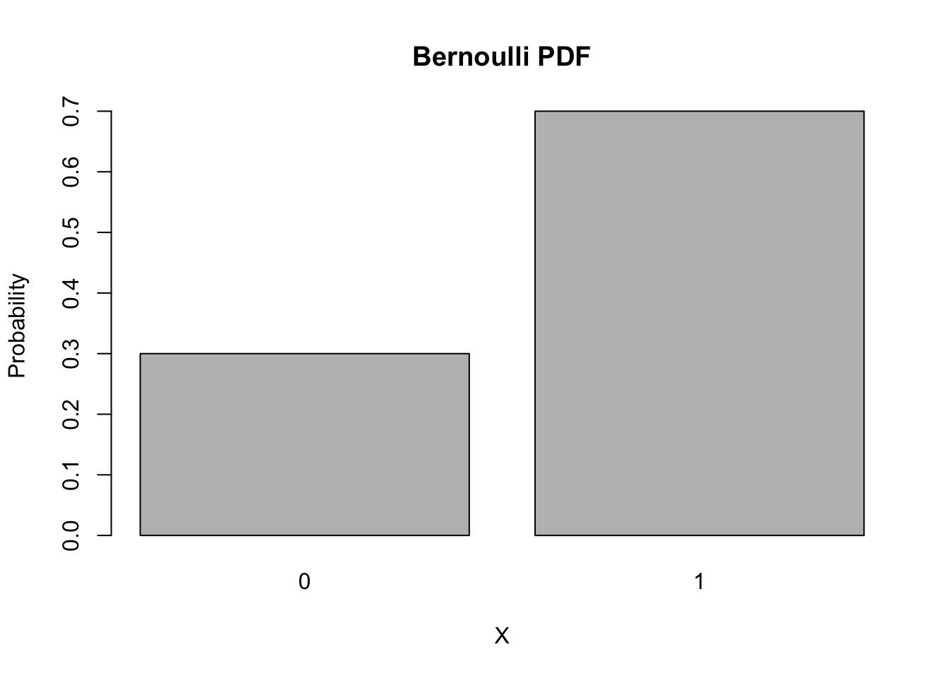
The Bernoulli has a very simple PDF,$$Pr(X=x)=\{\begin{array}{cc}p& x=1\\ 1-p& x=0\end{array}.$$This time, we’ll use the density function inside a barplot command, to send it directly to a plot.

barplot(names.arg = 0:1, 
        height = dbinom(0:1, size = 1, p = 0.7),
        main = "Bernoulli PDF", xlab = 'X', ylab = 'Probability')

Cumulative Distribution Functions: pbinom

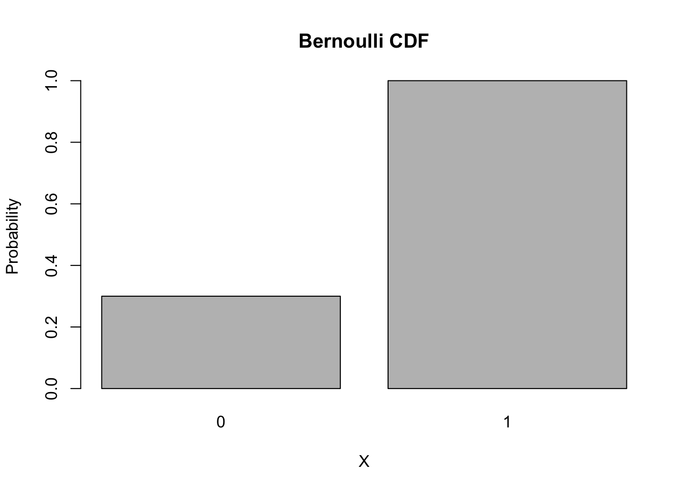
The CDF of a Bernoulli random variable is also simple.

barplot(names.arg = 0:1, 
        height = pbinom(0:1, size = 1, p = 0.7),
        main = "Bernoulli CDF", xlab = 'X', ylab = 'Probability')