Processing of GNSS data collected on an airplane requires special handling of the troposphere. Due to large variations in altitude, the a priori hydrostatic and wet delays must be regularly updated since the tropospheric zenith delay (TZD) process noise would not allow proper tracking of those variations. However, the temperature and pressure reduction schemes employed in GPT2 do not seem well suited for this purpose, as demonstrated herein using data from the NGS kinematic challenge.
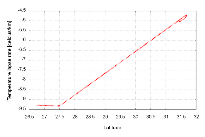
For temperature reduction, the GPT2 model [Lagler et al., 2013] replaced the constant lapse rate of -6.5⁰C/km by lapse rates dependent on location. Figure 1 below shows the interpolated temperature lapse rate as a function of the airplane latitude, for altitudes between 10 and 11.5 km. The rapid airplane displacements clearly emphasize that nearby grid points were assigned very different lapse rate values. While this is not an issue at sea level for a static receiver, when the airplane is flying at an altitude of 11 km, the differences in temperatures become very significant and impact wet zenith delay computations.
Figure 1: Temperature lapse rate provided by GPT2 as a function of latitude, for altitudes between 10 km and 11.5 km.
As opposed to the GPT model, GPT2 also provides values for the predicted water vapor pressure, although this measure only seems valid at the altitude of the grid points. For high altitudes, the water vapor pressure given exceeds the saturation vapor pressure, leading to a relative humidity greater than 100%. The pressure reduction process is based on a virtual temperature, also dependent on the water vapor pressure, and provides values significantly different from GPT at high altitudes.
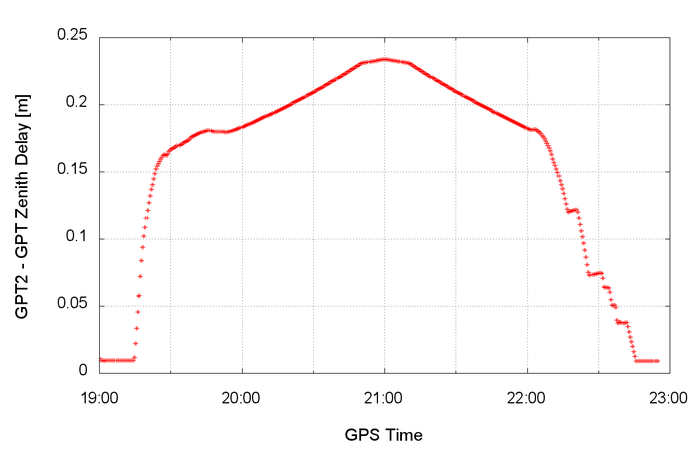
The combined effect of incorrect temperature, pressure and water vapor on the total zenith delay is depicted in Figure 2, showing differences with the GPT model. Large differences reaching more than 20 cm exist between models, and the consequences on the PPP solution are obviously disastrous…
Figure 2: Differences in total zenith delay between GPT2 and GPT.
Perhaps that the GPT2 model may never have been intended to be used in such applications, and perhaps that if I had understood the model before blindly using it, I wouldn’t have been surprised by the results. My suggestion is still to put a note in the GPT2 source code on those shortcomings, which would save (de)buggers like me a few days of work.
Reference
Lagler, K., M. Schindelegger, J. Böhm, H. Krásná, and T. Nilsson (2013), GPT2: Empirical slant delay model for radio space geodetic techniques, Geophys. Res. Lett., 40, 1069–1073, doi:10.1002/grl.50288.
Obtaining mm-level positioning accuracies with GNSS requires modeling of all error sources such as higher-order ionospheric effects. As a part of an IAG working group, I collaborated with European colleagues to investigate how this error source could be estimated as a part of the PPP filter. The results were published last week in GPS Solutions (Banville et al. 2017).
The idea behind this project came from a paper by Zehentner and Mayer-Guërr (2016) who estimated higher-order ionospheric effects within their PPP filter for LEO orbit determination. Since both the first- and second-order effects are linearly dependent on the slant total electron content (STEC), it is possible to modify the partial derivatives of the STEC parameters in the PPP filter to effectively estimate both terms jointly into a single parameter. This new processing strategy was however not the focus of their paper and they provided very little insights into the method. Hence, we decided to verify if this methodology is indeed applicable and under which circumstances.
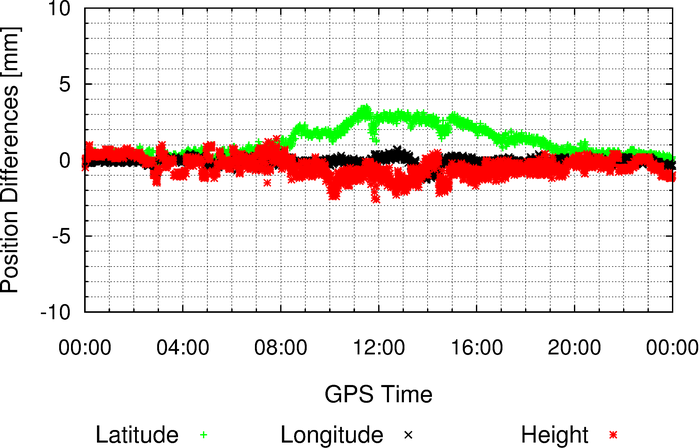
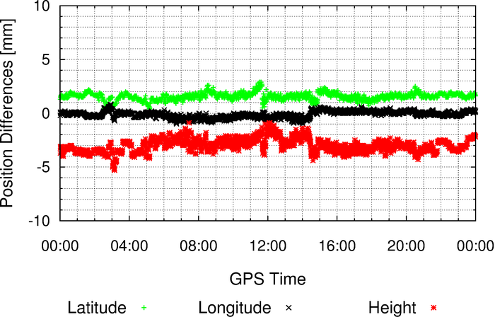
As an example, I will present results from station HERS with data collected on 8 November 2001, a day with high ionospheric activity. The first thing we were interested in was to measure the impact of higher-order ionospheric effects on kinematic PPP position estimates. The following figure shows position differences between two kinematic PPP solutions: one with second- and third-order ionospheric corrections applied (using the RINEX_HO utility) and another one without any of these corrections applied.
Fig 1 Impact of higher-order ionospheric effects on kinematic PPP
As we can see, differences are at the millimeter level and affect mainly the latitude component, with a peak error around 3 mm. I have to admit that this is quite tiny and that it is not perceptible in the original kinematic PPP time series since it is buried in the noise of the solution. It is only when differencing solutions that we can start to isolate the impact of this error source. In static mode, the impact is even less pronounced: it can be approximated by taking the mean of the time series in the above figure. Hence, we are talking about a latitude error of 1 mm or less over a 24-hour session.
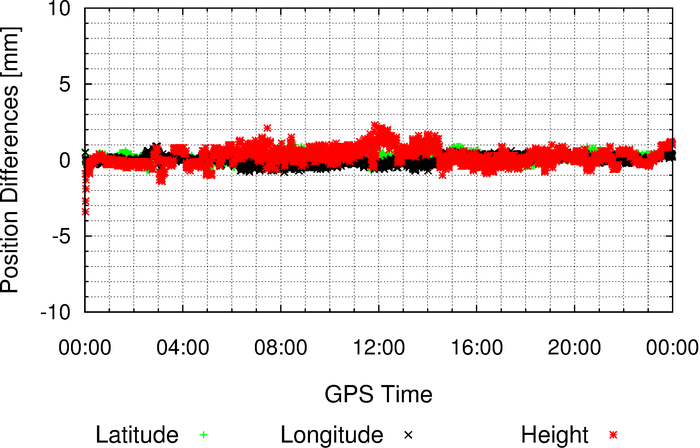
In the next step, we modified the partial derivatives in the PPP filter to estimate both first- and second-order ionospheric effects, as described above. Fig 2 presents the difference in kinematic PPP solutions between this new approach and the RINEX_HO solution:
Fig 2 Errors introduced when neglecting the receiver DCB in the PPP filter
The new approach introduced biases of a few millimeters in the position estimates. The magnitude of these biases exceeds the position errors caused by higher-order ionospheric effects, which is quite concerning. These biases originate from the definition of the estimable parameters in the PPP filter: slant ionospheric delays in PPP are contaminated by the receiver DCB. Since every satellite now has slightly different partial derivatives for the STEC parameters, the receiver DCB propagates into the position estimates; the larger the receiver DCB, the larger the position biases.
To solve this issue, we need to estimate unbiased STEC. This can be achieved in two ways: either by using a mathematical representation of VTEC or by introducing external constraints from a global ionospheric map (GIM). With the latter approach, the two kinematic PPP solutions now agree fairly well:
Fig 3 With proper handling of the receiver DCB, the PPP solution performs to the same level as the RINEX_HO solution
In conclusion, it is indeed possible to estimate higher-order ionospheric effects directly within the PPP filter. However, we still need GIMs to isolate the receiver DCB which goes a little bit against the initial purpose of this approach which was to estimate STEC without relying on external inputs. For all the details, please read the full paper!
References
Banville S, Sieradzki R, Hoque M, Wezka K, Hadas T (2017) On the estimation of higher-order ionospheric effects in precise point positioning. GPS Solut doi:10.1007/s10291-017-0655-0
Zehentner N, Mayer-Gu¨rr T (2016) Precise orbit determination based on raw GPS measurements. J Geod 90:275–286. doi:10.1007/s00190-015-0872-7