
一、节点电压方程出发点
进一步减少方程数,用未知的节点电压代替未知的支路电压来建立方程。
图3.2-1电路共有4个节点、 6条支路(把电流源和电导并联的电路看成是一条支路)。用支路电流法计算,需列写6个独立的方程

选取节点d为参考点,d点的电位为![]() ,则节点a、b、c为独立的节点,它们与d点之间的电压称为各节点的节点电压(node voltage),实际上就是各点的电位。这样a、b、c的节点电压是
,则节点a、b、c为独立的节点,它们与d点之间的电压称为各节点的节点电压(node voltage),实际上就是各点的电位。这样a、b、c的节点电压是![]() 。
。
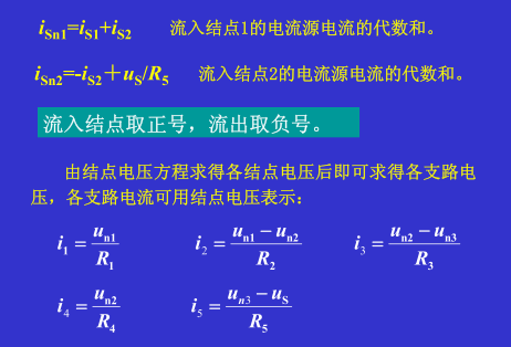
各电导支路的支路电流也就可用节点电压来表示
 |
结 论:用3个节点电压表示了6个支路电压。进一步减少了方程数。
1、节点电压方程
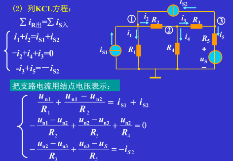
根据KCL,可得图3.2-1电路的节点电压方程

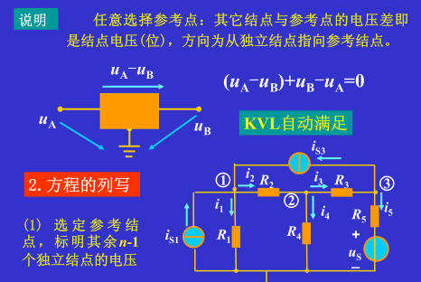
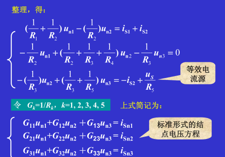
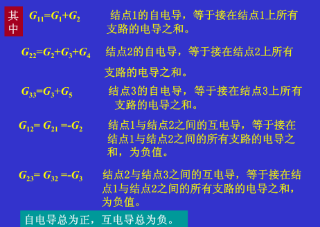
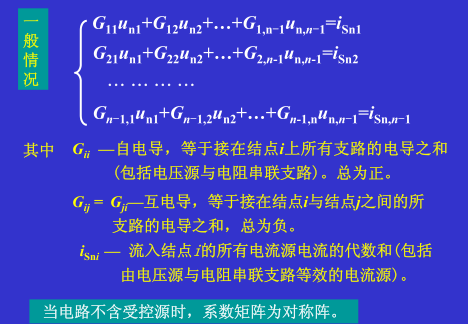
节点电压方程的一般形式
自电导×本节点电压-Σ(互电导×相邻节点电压)= 流入本节点的所有电流源的电流的代数和
自电导(self conductance)是指与每个节点相连的所有电导之和,互电导(mutual conductance)是指连接两个节点之间的支路电导。
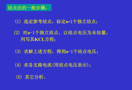
节点电压法分析电路的一般步骤
确定参考节点,并给其他独立节点编号。列写节点电压方程,并求解方程,求得各节点电压。由求得的节点电压,再求其他的电路变量,如支路电流、电压等。
例3.2-1 图3.2-1所示电路中,G1=G2=G3=2S,G4=G5=G6=1S,![]() ,
,![]() ,求各支路电流。
,求各支路电流。
解:1. 电路共有4个节点,选取d为参考点,![]() 。其他三个独立节点的节点电压分别为
。其他三个独立节点的节点电压分别为![]() 。
。
2. 列写节点电压方程
节点a: ![]()
节点b: ![]()
节点c: ![]()
代入参数,并整理,得到

解方程,得
![]()
3. 求各支路电流

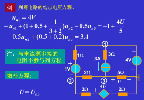
特 别 注 意:节点电压方程的本质是KCL,即Σ(流出电流) =Σ(流入电流),在节点电压方程中,方程的左边是与节点相连的电导上流出的电流之和,方程的右边则是与节点相连的电流源流入该节点的电流之和。如果某个电流源上还串联有一个电导,那么该电导就不应再计入自电导和互电导之中,因为该电导上的电流(与它串联的电流源的电流)已经计入方程右边了。
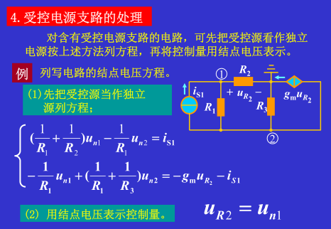
例3.2-2 图3.2-2所示电路,试列出它的节点电压方程。

解:对于节点a,流入的电流源![]() 的支路上还串联了一个电阻R1,在计算a点的自电导时,不应再把R1计算进去,所以a点的节点电压方程为
的支路上还串联了一个电阻R1,在计算a点的自电导时,不应再把R1计算进去,所以a点的节点电压方程为
![]()
b点的节点电压方程为
![]()
2、弥尔曼定理
当电路只有两个节点时,这种电路称为单节偶电路(single node-pair circuit)。对于单节偶电路,有弥尔曼定理。
弥尔曼定理:对于只有两个节点的单节偶电路,节偶电压等于流入独立节点的所有电流源电流的代数和除以节偶中所有电导之和。
![]()
二、含有电压源的电路
1、有伴电压源
结 论:如果电路中的电压源是有伴电压源,将有伴电压源等效成有伴电流源。
方法一 把电压源当电流源处理
把电压源当作电流源看待,并设定电压源的电流,列写节点电压方程。利用“电压源的电压等于其跨接的两个独立节点的节点电压之差”这个关系,再补充一个方程式,联立求解。
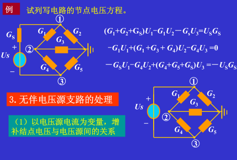
2、无伴电压源
电压源的一端与参考点相连
结 论
电压源一端与参考点相连,另一端的节点电压就是电压源的电压,节点电压方程减少一个。
方法二 超节点(super node)方法
虚线框当作一个超节点处理,列写节点电压方程。
注 意:列写这个超节点的方程时,其中的“自电导×本节点电压”这一项应包括两个部分,即组成该超节点的每个节点的电压与其相应的自电导的乘积。
 |
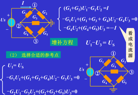
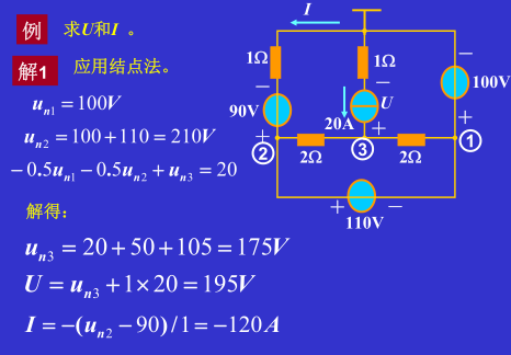
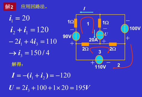
例3.2-3 图3.2-3所示电路,试列出它的节点电压方程,并求出电流I。
解:选取a、b、c为独立节点,由于6V无伴电压源的一端与参考点相连,所以c点的节点电压为
![]() (1)
(1)
对于节点a: ![]() (2)
(2)
对于节点b: ![]() (3)
(3)
将(1)式代入(2)、(3)式,并整理,得到

解得: ![]()
所以, ![]()
2)电压源的两端都不与参考点相连
例3.2-4 图3.2-4所示电路,![]() ,用节点电压法计算各电阻上的电压。
,用节点电压法计算各电阻上的电压。
 |
解:电路中含有两个电压源,相互之间又无公共端,所以只有一个电压源的一端可以连到参考点,而另一电压源的两端都不能与参考点相连。
选取1V电压源的正极为参考点,并标出其他独立节点a、b、c,如图3.2-5所示。这样,
![]() (1)
(1)
3.6V电压源的两端都不与参考点相连,跨接于节点a、c之间,设它的电流为I,并把它当作电流源处理。
对于节点a: ![]() (2)
(2)
对于节点c: ![]() (3)
(3)
代入参数,并整理(1)、(2)、(3)式,得
![]() (4)
(4)
再补充电压源的方程: ![]() (5)
(5)
解得: ![]() 。
。
所以,各电阻上的电压为

利用超节点的方法计算例3.2-4。
对超节点: ![]()
对节点b: ![]()
另外,对3.6V的电压源: ![]()
代入参数,并整理,得
![]()
解得: ![]()
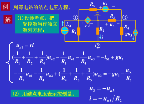
三、含有受控源电路
思 路:电路中含有受控源时,将受控源当独立源处理,列写节点电压方程。当然,当受控源的控制量不是某个节点的节点电压时,还需补充一个反映控制量与节点电压之间关系的方程式。

例3.2-5 电路如图3.2-5(a)所示,求电流I。
解:电路中含有一受控电流源,将它当作独立电流源看待。另外还有一个有伴电压源,将该有伴电压源等效成有伴电流源,等效电路如图3.2-6(b)所示。
对节点a: ![]()
对节点b: ![]()
又 ![]()
经整理后,得到

解得: ![]()
所以,电流 ![]()
快来看看英文的节点电压法:
来源:https://www.allaboutcircuits.com/textbook/direct-current/chpt-10/node-voltage-method/
Node Voltage Method
Chapter 10 - DC Network Analysis
The node voltage method of analysis solves for unknown voltages at circuit nodes in terms of a system of KCL equations. This analysis looks strange because it involves replacing voltage sources with equivalent current sources. Also, resistor values in ohms are replaced by equivalent conductances in siemens, G = 1/R. The siemens (S) is the unit of conductance, having replaced the mho unit. In any event S = Ω-1. And S = mho (obsolete).
Method for Node Voltage Calculation
We start with a circuit having conventional voltage sources. A common node E0 is chosen as a reference point. The node voltages E1 and E2 are calculated with respect to this point.
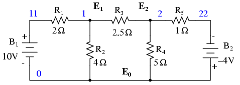
A voltage source in series with a resistance must be replaced by an equivalent current source in parallel with the resistance. We will write KCL equations for each node. The right hand side of the equation is the value of the current source feeding the node.
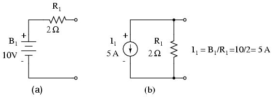
Replacing voltage sources and associated series resistors with equivalent current sources and parallel resistors yields the modified circuit. Substitute resistor conductances in siemens for resistance in ohms.
I1 = E1/R1 = 10/2 = 5 A I2 = E2/R5 = 4/1 = 4 A G1 = 1/R1 = 1/2 Ω = 0.5 S G2 = 1/R2 = 1/4 Ω = 0.25 S G3 = 1/R3 = 1/2.5 Ω = 0.4 S G4 = 1/R4 = 1/5 Ω = 0.2 S G5 = 1/R5 = 1/1 Ω = 1.0 S

The parallel conductances (resistors) may be combined by addition of the conductances. Though, we will not redraw the circuit. The circuit is ready for application of the node voltage method.
GA = G1 + G2 = 0.5 S + 0.25 S = 0.75 S GB = G4 + G5 = 0.2 S + 1 S = 1.2 S
Deriving a general node voltage method, we write a pair of KCL equations in terms of unknown node voltages V1 and V2 this one time. We do this to illustrate a pattern for writing equations by inspection.
GAE1 + G3(E1 - E2) = I1 (1) GBE2 - G3(E1 - E2) = I2 (2) (GA + G3 )E1 -G3E2 = I1 (1) -G3E1 + (GB + G3)E2 = I2 (2)
The coefficients of the last pair of equations above have been rearranged to show a pattern. The sum of conductances connected to the first node is the positive coefficient of the first voltage in equation (1). The sum of conductances connected to the second node is the positive coefficient of the second voltage in equation (2). The other coefficients are negative, representing conductances between nodes. For both equations, the right hand side is equal to the respective current source connected to the node. This pattern allows us to quickly write the equations by inspection. This leads to a set of rules for the node voltage method of analysis.
Node Voltage Rules:
Convert voltage sources in series with a resistor to an equivalent current source with the resistor in parallel.
Change resistor values to conductances.
Select a reference node(E0)
Assign unknown voltages (E1)(E2) ... (EN)to remaining nodes.
Write a KCL equation for each node 1,2, ... N. The positive coefficient of the first voltage in the first equation is the sum of conductances connected to the node. The coefficient for the second voltage in the second equation is the sum of conductances connected to that node. Repeat for coefficient of third voltage, third equation, and other equations. These coefficients fall on a diagonal.
All other coefficients for all equations are negative, representing conductances between nodes. The first equation, second coefficient is the conductance from node 1 to node 2, the third coefficient is the conductance from node 1 to node 3. Fill in negative coefficients for other equations.
The right hand side of the equations is the current source connected to the respective nodes.
Solve system of equations for unknown node voltages.
Example: Set up the equations and solve for the node voltages using the numerical values in the above figure.
Solution:
(0.5+0.25+0.4)E1 -(0.4)E2= 5 -(0.4)E1 +(0.4+0.2+1.0)E2 = -4 (1.15)E1 -(0.4)E2= 5 -(0.4)E1 +(1.6)E2 = -4 E1 = 3.8095 E2 = -1.5476
The solution of two equations can be performed with a calculator, or with octave (not shown).[octav] The solution is verified with SPICE based on the original schematic diagram with voltage sources. [spi] Though, the circuit with the current sources could have been simulated.
V1 11 0 DC 10 V2 22 0 DC -4 r1 11 1 2 r2 1 0 4 r3 1 2 2.5 r4 2 0 5 r5 2 22 1 .DC V1 10 10 1 V2 -4 -4 1 .print DC V(1) V(2) .end v(1) v(2) 3.809524e+00 -1.547619e+00
One more example. This one has three nodes. We do not list the conductances on the schematic diagram. However, G1 = 1/R1, etc.
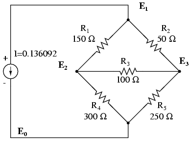
There are three nodes to write equations for by inspection. Note that the coefficients are positive for equation (1) E1, equation (2) E2, and equation (3) E3. These are the sums of all conductances connected to the nodes. All other coefficients are negative, representing a conductance between nodes. The right hand side of the equations is the associated current source, 0.136092 A for the only current source at node 1. The other equations are zero on the right hand side for lack of current sources. We are too lazy to calculate the conductances for the resistors on the diagram. Thus, the subscripted G’s are the coefficients.
(G1 + G2)E1 -G1E2 -G2E3 = 0.136092 -G1E1 +(G1 + G3 + G4)E2 -G3E3 = 0 -G2E1 -G3E2 +(G2 + G3 + G5)E3 = 0
We are so lazy that we enter reciprocal resistances and sums of reciprocal resistances into the octave “A” matrix, letting octave compute the matrix of conductances after “A=”.[octav] The initial entry line was so long that it was split into three rows. This is different than previous examples. The entered “A” matrix is delineated by starting and ending square brackets. Column elements are space separated. Rows are “new line” separated. Commas and semicolons are not need as separators. Though, the current vector at “b” is semicolon separated to yield a column vector of currents.
octave:12> A = [1/150+1/50 -1/150 -1/50 > -1/150 1/150+1/100+1/300 -1/100 > -1/50 -1/100 1/50+1/100+1/250] A = 0.0266667 -0.0066667 -0.0200000 -0.0066667 0.0200000 -0.0100000 -0.0200000 -0.0100000 0.0340000 octave:13> b = [0.136092;0;0] b = 0.13609 0.00000 0.00000 octave:14> x=A\b x = 24.000 17.655 19.310
Note that the “A” matrix diagonal coefficients are positive, That all other coefficients are negative.
The solution as a voltage vector is at “x”. E1 = 24.000 V, E2 = 17.655 V, E3 = 19.310 V. These three voltages compare to the previous mesh current and SPICE solutions to the unbalanced bridge problem. This is no coincidence, for the 0.13609 A current source was purposely chosen to yield the 24 V used as a voltage source in that problem.
Summary
Given a network of conductances and current sources, the node voltage method of circuit analysis solves for unknown node voltages from KCL equations.
See rules above for details in writing the equations by inspection.
The unit of conductance G is the siemens S. Conductance is the reciprocal of resistance: G = 1/R

