
试试读下诺顿定理英文资料:
来源于:https://www.allaboutcircuits.com/textbook/direct-current/chpt-10/nortons-theorem/
Norton’s Theorem
Chapter 10 - DC Network Analysis
What is Norton’s Theorem?
Norton’s Theorem states that it is possible to simplify any linear circuit, no matter how complex, to an equivalent circuit with just a single current source and parallel resistance connected to a load. Just as with Thevenin’s Theorem, the qualification of “linear” is identical to that found in the Superposition Theorem: all underlying equations must be linear (no exponents or roots).
Simplifying Linear Circuits
Contrasting our original example circuit against the Norton equivalent: it looks something like this:
. . . after Norton conversion . . .

Remember that a current source is a component whose job is to provide a constant amount of current, outputting as much or as little voltage necessary to maintain that constant current.
Thevenin’s Theorem vs. Norton’s Theorem
As with Thevenin’s Theorem, everything in the original circuit except the load resistance has been reduced to an equivalent circuit that is simpler to analyze. Also similar to Thevenin’s Theorem are the steps used in Norton’s Theorem to calculate the Norton source current (INorton) and Norton resistance (RNorton).
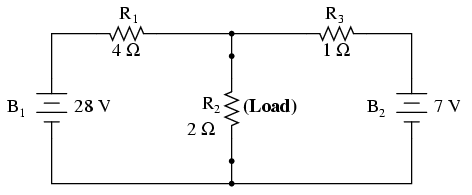
As before, the first step is to identify the load resistance and remove it from the original circuit:
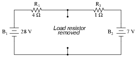
Then, to find the Norton current (for the current source in the Norton equivalent circuit), place a direct wire (short) connection between the load points and determine the resultant current. Note that this step is exactly opposite the respective step in Thevenin’s Theorem, where we replaced the load resistor with a break (open circuit):

With zero voltage dropped between the load resistor connection points, the current through R1 is strictly a function of B1‘s voltage and R1‘s resistance: 7 amps (I=E/R). Likewise, the current through R3 is now strictly a function of B2‘s voltage and R3‘s resistance: 7 amps (I=E/R). The total current through the short between the load connection points is the sum of these two currents: 7 amps + 7 amps = 14 amps. This figure of 14 amps becomes the Norton source current (INorton) in our equivalent circuit:

Remember, the arrow notation for a current source points in the direction opposite that of electron flow. Again, apologies for the confusion. For better or for worse, this is standard electronic symbol notation. Blame Mr. Franklin again!
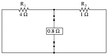
To calculate the Norton resistance (RNorton), we do the exact same thing as we did for calculating Thevenin resistance (RThevenin): take the original circuit (with the load resistor still removed), remove the power sources (in the same style as we did with the Superposition Theorem: voltage sources replaced with wires and current sources replaced with breaks), and figure total resistance from one load connection point to the other:
Now our Norton equivalent circuit looks like this:

If we re-connect our original load resistance of 2 Ω, we can analyze the Norton circuit as a simple parallel arrangement:

As with the Thevenin equivalent circuit, the only useful information from this analysis is the voltage and current values for R2; the rest of the information is irrelevant to the original circuit. However, the same advantages seen with Thevenin’s Theorem apply to Norton’s as well: if we wish to analyze load resistor voltage and current over several different values of load resistance, we can use the Norton equivalent circuit again and again, applying nothing more complex than simple parallel circuit analysis to determine what’s happening with each trial load.
REVIEW:
•Norton’s Theorem is a way to reduce a network to an equivalent circuit composed of a single current source, parallel resistance, and parallel load.
•Steps to follow for Norton’s Theorem:
•(1) Find the Norton source current by removing the load resistor from the original circuit and calculating current through a short (wire) jumping across the open connection points where the load resistor used to be.
•(2) Find the Norton resistance by removing all power sources in the original circuit (voltage sources shorted and current sources open) and calculating total resistance between the open connection points.
•(3) Draw the Norton equivalent circuit, with the Norton current source in parallel with the Norton resistance. The load resistor re-attaches between the two open points of the equivalent circuit.
•(4) Analyze voltage and current for the load resistor following the rules for parallel circuits.

