
英文的戴维南定理
来源于:https://www.allaboutcircuits.com/textbook/direct-current/chpt-10/thevenins-theorem/
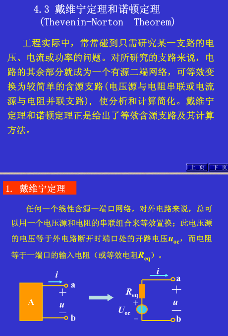
Thevenin’s Theorem
Chapter 10 - DC Network Analysis
Thevenin’s Theorem states that it is possible to simplify any linear circuit, no matter how complex, to an equivalent circuit with just a single voltage source and series resistance connected to a load. The qualification of “linear” is identical to that found in the Superposition Theorem, where all the underlying equations must be linear (no exponents or roots). If we’re dealing with passive components (such as resistors, and later, inductors and capacitors), this is true. However, there are some components (especially certain gas-discharge and semiconductor components) which are nonlinear: that is, their opposition to current changes with voltage and/or current. As such, we would call circuits containing these types of components, nonlinear circuits.
Thevenin’s Theorem is especially useful in analyzing power systems and other circuits where one particular resistor in the circuit (called the “load” resistor) is subject to change, and re-calculation of the circuit is necessary with each trial value of load resistance, to determine voltage across it and current through it. Let’s take another look at our example circuit:
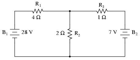
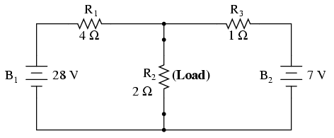
Let’s suppose that we decide to designate R2 as the “load” resistor in this circuit. We already have four methods of analysis at our disposal (Branch Current, Mesh Current, Millman’s Theorem, and Superposition Theorem) to use in determining voltage across R2 and current through R2, but each of these methods are time-consuming. Imagine repeating any of these methods over and over again to find what would happen if the load resistance changed (changing load resistance is very common in power systems, as multiple loads get switched on and off as needed. the total resistance of their parallel connections changing depending on how many are connected at a time). This could potentially involve a lot of work!
Thevenin’s Theorem makes this easy by temporarily removing the load resistance from the original circuit and reducing what’s left to an equivalent circuit composed of a single voltage source and series resistance. The load resistance can then be re-connected to this “Thevenin equivalent circuit” and calculations carried out as if the whole network were nothing but a simple series circuit:
. . . after Thevenin conversion . . .
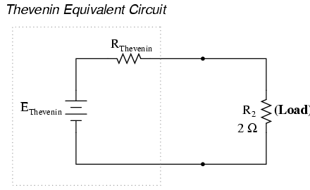
The “Thevenin Equivalent Circuit” is the electrical equivalent of B1, R1, R3, and B2 as seen from the two points where our load resistor (R2) connects.
The Thevenin equivalent circuit, if correctly derived, will behave exactly the same as the original circuit formed by B1, R1, R3, and B2. In other words, the load resistor (R2) voltage and current should be exactly the same for the same value of load resistance in the two circuits. The load resistor R2 cannot “tell the difference” between the original network of B1, R1, R3, and B2, and the Thevenin equivalent circuit of EThevenin, and RThevenin, provided that the values for EThevenin and RThevenin have been calculated correctly.
The advantage in performing the “Thevenin conversion” to the simpler circuit, of course, is that it makes load voltage and load current so much easier to solve than in the original network. Calculating the equivalent Thevenin source voltage and series resistance is actually quite easy. First, the chosen load resistor is removed from the original circuit, replaced with a break (open circuit):
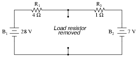
Next, the voltage between the two points where the load resistor used to be attached is determined. Use whatever analysis methods are at your disposal to do this. In this case, the original circuit with the load resistor removed is nothing more than a simple series circuit with opposing batteries, and so we can determine the voltage across the open load terminals by applying the rules of series circuits, Ohm’s Law, and Kirchhoff’s Voltage Law:
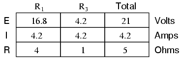
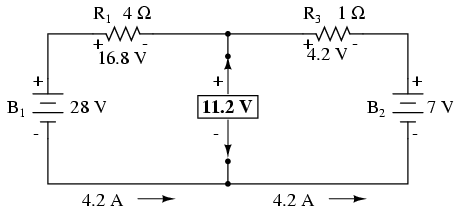
The voltage between the two load connection points can be figured from the one of the battery’s voltage and one of the resistor’s voltage drops, and comes out to 11.2 volts. This is our “Thevenin voltage” (EThevenin) in the equivalent circuit:
To find the Thevenin series resistance for our equivalent circuit, we need to take the original circuit (with the load resistor still removed), remove the power sources (in the same style as we did with the Superposition Theorem: voltage sources replaced with wires and current sources replaced with breaks), and figure the resistance from one load terminal to the other:
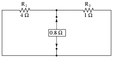
With the removal of the two batteries, the total resistance measured at this location is equal to R1 and R3 in parallel: 0.8 Ω. This is our “Thevenin resistance” (RThevenin) for the equivalent circuit:
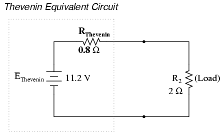
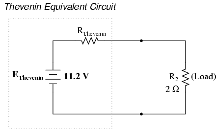
With the load resistor (2 Ω) attached between the connection points, we can determine voltage across it and current through it as though the whole network were nothing more than a simple series circuit:
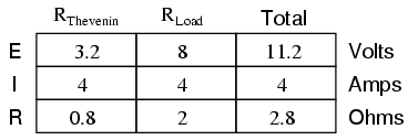
Notice that the voltage and current figures for R2 (8 volts, 4 amps) are identical to those found using other methods of analysis. Also notice that the voltage and current figures for the Thevenin series resistance and the Thevenin source (total) do not apply to any component in the original, complex circuit. Thevenin’s Theorem is only useful for determining what happens to a single resistor in a network: the load.
The advantage, of course, is that you can quickly determine what would happen to that single resistor if it were of a value other than 2 Ω without having to go through a lot of analysis again. Just plug in that other value for the load resistor into the Thevenin equivalent circuit and a little bit of series circuit calculation will give you the result.
REVIEW:
Thevenin’s Theorem is a way to reduce a network to an equivalent circuit composed of a single voltage source, series resistance, and series load.
Steps to follow for Thevenin’s Theorem:
(1) Find the Thevenin source voltage by removing the load resistor from the original circuit and calculating voltage across the open connection points where the load resistor used to be.
(2) Find the Thevenin resistance by removing all power sources in the original circuit (voltage sources shorted and current sources open) and calculating total resistance between the open connection points.
(3) Draw the Thevenin equivalent circuit, with the Thevenin voltage source in series with the Thevenin resistance. The load resistor re-attaches between the two open points of the equivalent circuit.
(4) Analyze voltage and current for the load resistor following the rules for series circuits.

